word2vec
谷歌2013年提出的word2vec是目前最常用的词嵌入模型之一。Word2ec实际是一种浅层的神经网络模型,它有两种网络结构,分别是CBOW( Continues Bag of words)和 Skip-gram。
百面 Word2Vec
问 Word2Vec是如何工作的?
答:CBOW的目标是根据上下文出现的词语来预测当前词的生成概率,如图1.3 (a) 所示;而Skip-gram是根据当前词来预测上下文中各词的生成概率,如图1.3 (b)所示。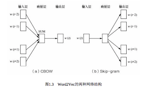
其中w(t)是当前所关注的词,w(t-2)、 w(t-1)、 w(t+1)、 w(t+2)是 上下文中出现的词。这里前后滑动窗口大小均设为2。
CBOW和Skip-gram都可以表示成由输入层(Input)、映射层(Projection)和输出层(Output)组成的神经网络。
输入层中的每个词由独热编码方式表示,即所有词均表示成一个N维向量,其中N为词汇表中单词的总数。在向量中,每个词都将与之对应的维度置为1,其余维度的值均设为0。
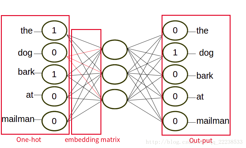
在映射层(又称隐含层)中,K个隐含单元( Hidden units)的取值可以由N维输入向量以及连接输入和隐含单元之间的N乘K维权重矩阵计算得到。在CBOV中,还需要将各个输入词所计算出的隐含单元求和。补一个其他博客的图。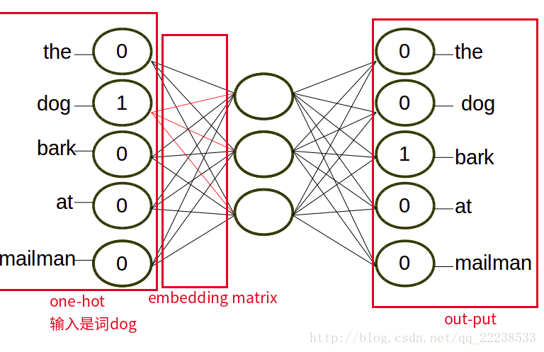
同理,输出层向量的值可以通过隐含层向量(K维),以及连接隐含层和输出层之间的KxN维权重矩阵计算得到。输出层也是一个N维向量,每维与词汇表中的一个单词相对应。最后,对输出层向量应用Softmax激活函数,可以计算出每个单词的生成概率。Softmax激活函数的定义为: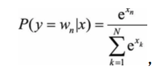
其中x代表N维的原始输出向量,xn为在原始输出向量中,与单词wn所对应维度的取值。
接下来的任务就是训练神经网络的权重,使得语料库中所有单词的整体生成概率最大化。从输入层到隐含层需要一个维度为NxK的权重矩阵,从隐含层到输出层又需要一个维度为KxN的权重矩阵,学习权重可以用反向传播算法实现,每次迭代时将权重沿梯度更优的方向进行一小步更新。但是由于Softmax激活函数中存在归一化项的缘故,推导出来的迭代公式需要对词汇表中的所有单词进行遍历,使得每次迭代过程非常缓慢,由此产生了Hierarchical Softmax和Negative Sampling两种改进方法。训练得到维度为NxK和KxN的两个权重矩阵之后,可以选择其中一个作为N个词的K维向量表示。
王喆 知乎
万物皆Embedding,从经典的word2vec到深度学习基本操作item2vec - 知乎
万物皆Embedding,从经典的word2vec到深度学习基本操作item2vec
什么是embedding?
简单来说,embedding就是用一个低维的向量表示一个物体,可以是一个词,或是一个商品,或是一个电影等等。这个embedding向量的性质是能使距离相近的向量对应的物体有相近的含义,比如 Embedding(复仇者联盟)和Embedding(钢铁侠)之间的距离就会很接近,但 Embedding(复仇者联盟)和Embedding(乱世佳人)的距离就会远一些。
除此之外Embedding甚至还具有数学运算的关系,比如Embedding(马德里)-Embedding(西班牙)+Embedding(法国)≈Embedding(巴黎)
从另外一个空间表达物体,甚至揭示了物体间的潜在关系,从某种意义上来说,Embedding方法甚至具备了一些本体论的哲学意义。
为什么说embedding是深度学习的基本操作?
Embedding能够用低维向量对物体进行编码还能保留其含义的特点非常适合深度学习。在传统机器学习模型构建过程中,经常使用one hot encoding对离散特征,特别是id类特征进行编码,但由于one hot encoding的维度等于物体的总数,比如阿里的商品one hot encoding的维度就至少是千万量级的。这样的编码方式对于商品来说是极端稀疏的,甚至用multi hot encoding对用户浏览历史的编码也会是一个非常稀疏的向量。
而深度学习的特点以及工程方面的原因使其不利于稀疏特征向量的处理。因此如果能把物体编码为一个低维稠密向量再喂给DNN,自然是一个高效的基本操作。因为从梯度下降的过程来说,如果特征过于稀疏会导致整个网络收敛过慢,因为每次更新只有极少数的权重会得到更新。这样在样本有限的情况下会导致模型不收敛。而且还会导致全连接层有过多的参数。
尽管有采用relu函数等各种手段减少梯度消失现象的发生,但nn还是会存在梯度消失问题,所以到输入层的时候梯度受输出层diff的影响已经很小了因此收敛慢再加上大量稀疏特征导致一次只有个别权重更新这个现象就更严重了。对于lr来说,梯度能够直接传导到权重,因为其只有一层。倒不是说lr更适合处理大规模离散特征 而是相比nn 需要更少的数据收敛 如果数据量和时间都无限的话nn也适合处理稀疏特征。
McCormick W2V
http://mccormickml.com/2016/04/19/word2vec-tutorial-the-skip-gram-model/
The Model
Word2Vec uses a trick you may have seen elsewhere in machine learning. We’re going to train a simple neural network with a single hidden layer to perform a certain task, but then we’re not actually going to use that neural network for the task we trained it on! Instead, the goal is actually just to learn the weights of the hidden layer。
We’ll train the neural network to do this by feeding it word pairs found in our training documents.The word highlighted in blue is the input word.
this is skip-gram.
Model Details
let’s say we have a vocabulary of 10,000 unique words.We’re going to represent an input word as a one-hot vector. This vector will have 10,000 components.The output of the network is a single vector (also with 10,000 components) Here’s the architecture of our neural network.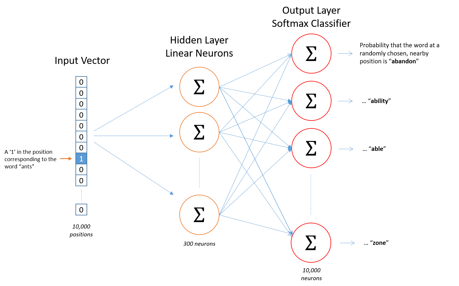
There is no activation function on the hidden layer neurons, but the output neurons use softmax.
When training this network on word pairs, the input is a one-hot vector representing the input word and the training output is also a one-hot vector representing the output word.But when you evaluate the trained network on an input word, the output vector will actually be a probability distribution (i.e., a bunch of floating point values, not a one-hot vector).
The Hidden Layer
For our example, we’re going to say that we’re learning word vectors with 300 features. So the hidden layer is going to be represented by a weight matrix with 10,000 rows (one for every word in our vocabulary) and 300 columns (one for every hidden neuron).The number of features is a “hyper parameter” that you would just have to tune to your application .
显然,每个单词对应一个300维的隐向量,也可以理解为300维的语义。
that is why we use one-hot .右边矩阵中绿色的值即为左边矩阵中1对应的词的隐向量。 对应的,竖着的第一列即为隐藏层第一个神经元连接的上一层的神经元权重。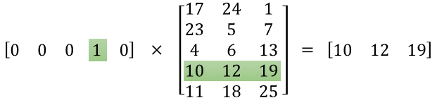
just as this image.根据反向传播公式,当梯度传递到这一层时,只有非0的值才会对梯度进行更新。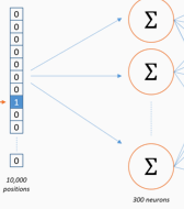
This means that the hidden layer of this model is really just operating as a lookup table. The output of the hidden layer is just the “word vector” for the input word.
Negative Sampling
The skip-gram neural network contains a huge number of weights… For our example with 300 features and a vocab of 10,000 words, that’s 3M weights in the hidden layer and output layer each! Training this on a large dataset would be prohibitive, And to make matters worse, you need a huge amount of training data in order to tune that many weights and avoid over-fitting. so the word2vec authors introduced a number of tweaks to make training feasible.The first one is Negative Sampling
the innovations:
- Subsampling frequent words to decrease the number of training examples.
- Modifying the optimization objective with a technique they called “Negative Sampling”, which causes each training sample to update only a small percentage of the model’s weights.
It’s worth noting that subsampling frequent words and applying Negative Sampling not only reduced the compute burden of the training process, but also improved the quality of their resulting word vectors as well.
Subsampling Frequent Words
The word highlighted in blue is the input word.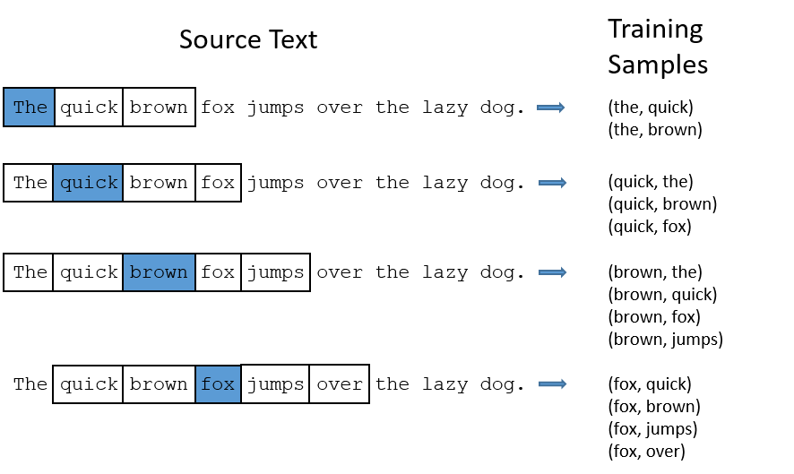
There are two “problems” with common words like “the”:
- When looking at word pairs, (“fox”, “the”) doesn’t tell us much about the meaning of “fox”. “the” appears in the context of pretty much every word.
- We will have many more samples of (“the”, …) than we need to learn a good vector for “the”.
Word2Vec implements a “subsampling” scheme to address this. For each word we encounter in our training text, there is a chance that we will effectively delete it from the text. The probability that we cut the word is related to the word’s frequency.
If we have a window size of 10, and we remove a specific instance of “the” from our text:
- As we train on the remaining words, “the” will not appear in any of their context windows.
- We’ll have 10 fewer training samples where “the” is the input word.
Sample rate
wi is the word, z(wi) is the fraction of the total words in the corpus that are that word. For example, if the word “peanut” occurs 1,000 times in a 1 billion word corpus, then z(‘peanut’) = 1E-6.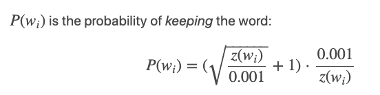
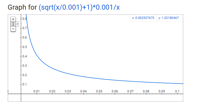
1.P(wi)=1.0 (100% chance of being kept) when z(wi)<=0.0026.
This means that only words which represent more than 0.26% of the total words will be subsampled.
2.P(wi)=0.5 (50% chance of being kept) when z(wi)=0.00746.
3.P(wi)=0.033 (3.3% chance of being kept) when z(wi)=1.0.
That is, if the corpus consisted entirely of word wi, which of course is ridiculous.
Negative Sampling
Negative sampling addresses this by having each training sample only modify a small percentage of the weights, rather than all of them. Here’s how it works.
When training the network on the word pair (“fox”, “quick”), recall that the “label” or “correct output” of the network is a one-hot vector. That is, for the output neuron corresponding to “quick” to output a 1, and for all of the other thousands of output neurons to output a 0.
With negative sampling, we are instead going to randomly select just a small number of “negative” words (let’s say 5) to update the weights for. (In this context, a “negative” word is one for which we want the network to output a 0 for). We will also still update the weights for our “positive” word (which is the word “quick” in our current example).
Recall that the output layer of our model has a weight matrix that’s 300 x 10,000. So we will just be updating the weights for our positive word (“quick”), plus the weights for 5 other words that we want to output 0. That’s a total of 6 output neurons, and 1,800 weight values total. That’s only 0.06% of the 3M weights in the output layer!
In the hidden layer, only the weights for the input word are updated (this is true whether you’re using Negative Sampling or not).
Selecting Negative Samples
The “negative samples” (that is, the 5 output words that we’ll train to output 0) are selected using a “unigram distribution”, where more frequent words are more likely to be selected as negative samples.
For instance, suppose you had your entire training corpus as a list of words, and you chose your 5 negative samples by picking randomly from the list. In this case, the probability for picking the word “couch” would be equal to the number of times “couch” appears in the corpus, divided the total number of word occus in the corpus. This is expressed by the following equation: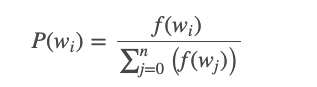
The authors state in their paper that they tried a number of variations on this equation, and the one which performed best was to raise the word counts to the 3/4 power: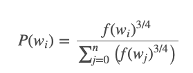
Applying word2vec to Recommenders and Advertising
The key principle behind word2vec is the notion that the meaning of a word can be inferred from it’s context–what words tend to be around it. To abstract that a bit, text is really just a sequence of words, and the meaning of a word can be extracted from what words tend to be just before and just after it in the sequence.
What researchers and companies are finding is that the time series of online user activity offers the same opportunity for inferring meaning from context. That is, as a user browses around and interacts with different content, the abstract qualities of a piece of content can be inferred from what content the user interacts with before and after. This allows ML teams to apply word vector models to learn good vector representations for products, content, and ads.
The word2vec approach has proven successful in extracting these hidden insights, and being able to compare, search, and categorize items on these abstract dimensions opens up a lot of opportunities for smarter, better recommendations.
Four Production Examples
Music Recommendations
One use is to create a kind of “music taste” vector for a user by averaging together the vectors for songs that a user likes to listen to. This taste vector can then become the query for a similarity search to find songs which are similar to the user’s taste vector.
and Listing Recommendations at Airbnb,Product Recommendations in Yahoo Mail,Matching Ads to Search Queries
几篇论文
Distributed Representations of Words and Phrases and their Compositionality
Google的Tomas Mikolov提出word2vec的两篇文章之一,这篇文章更具有综述性质,列举了NNLM、RNNLM等诸多词向量模型,但最重要的还是提出了CBOW和Skip-gram两种word2vec的模型结构。虽然词向量的研究早已有之,但不得不说还是Google的word2vec的提出让词向量重归主流,拉开了整个embedding技术发展的序幕。
Efficient Estimation of Word Representations in Vector Space
Tomas Mikolov的另一篇word2vec奠基性的文章。相比上一篇的综述,本文更详细的阐述了Skip-gram模型的细节,包括模型的具体形式和 Hierarchical Softmax和 Negative Sampling两种可行的训练方法。
Word2vec Parameter Learning Explained
虽然Mikolov的两篇代表作标志的word2vec的诞生,但其中忽略了大量技术细节,如果希望完全读懂word2vec的原理和实现方法,比如词向量具体如何抽取,具体的训练过程等,强烈建议大家阅读UMich Xin Rong博士的这篇针对word2vec的解释性文章。惋惜的是Xin Rong博士在完成这篇文章后的第二年就由于飞机事故逝世,在此也致敬并缅怀一下Xin Rong博士。