featexp
https://towardsdatascience.com/my-secret-sauce-to-be-in-top-2-of-a-kaggle-competition-57cff0677d3c
feature understanding
if target is binary, scatter is not very useful.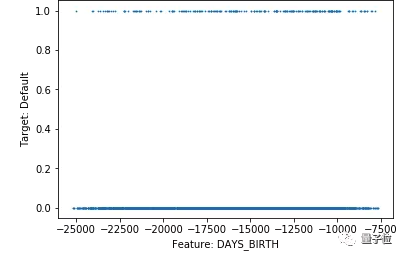
And for continuous target, too many data points make it difficult to understand the target vs. feature trend.
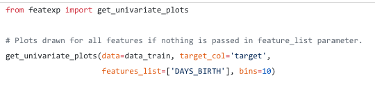
use above code,Featexp creates equal population bins (X-axis) of a numeric feature.It then calculates target’s mean in each bin and plots it in the left-hand side plot above. As you can see the plot on the right shows they are the same number.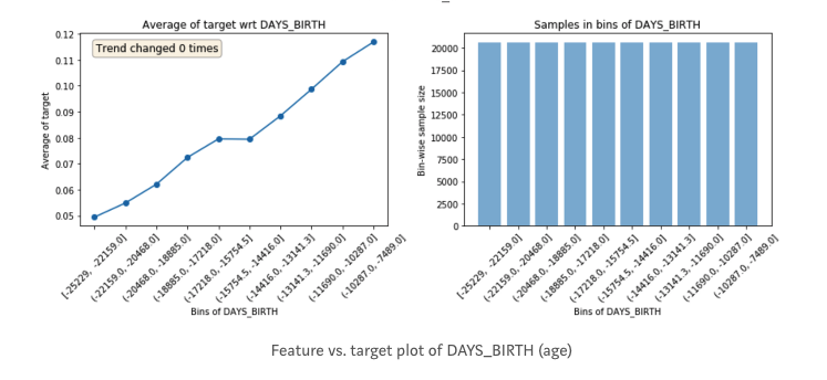
Identifying noisy features
Noisy features lead to overfitting and identifying them isn’t easy. In featexp, you can pass a test set and compare feature trends in train|test to identify noisy ones. This test set is not the actual test set. Its your local test set|validation set for which you know target.
get_univariate_plots(data=data_train, target_col=’target’, data_test=data_test, features_list=[‘DAYS_EMPLOYED’])
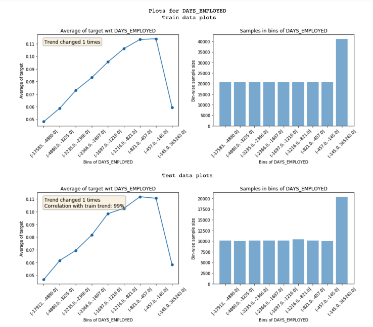
Featexp calculates two metrics to display on these plots which help with gauging(计量;测量) noisiness:
1.Trend correlation (seen in test plot): If a feature doesn’t hold same trend w.r.t. target across train and evaluation sets, it can lead to overfitting. This happens because the model is learning something which is not applicable in test data. Trend correlation helps understand how similar train/test trends are and mean target values for bins in train & test are used to calculate it. Feature above has 99% correlation. Doesn’t seem noisy!
2.Trend changes: Sudden and repeated changes in trend direction could imply noisiness. But, such trend change can also happen because that bin has a very different value in terms of other features and hence, its value can’t really be compared with other bins.
for example the nosiy feature.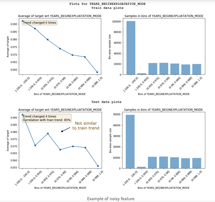
Dropping low trend-correlation features works well when there are a lot of features and they are correlated with each other. It leads to less overfitting and other correlated features avoid information loss. It’s also important to not drop too many important features as it might lead to a drop in performance. Also, you can’t identify these noisy features using feature importance because they could be fairly important and still be very noisy!
Using test data from a different time period works better because then you would be making sure if feature trend holds over time.
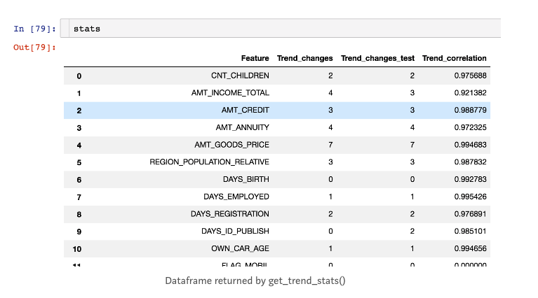
get_trend_stats() function in featexp returns a dataframe with trend correlation and changes for each feature.
from featexp import get_trend_stats stats=get_trend_stats(data=data_train,target_col=’target’,data_test=data_test)
try dropping features with low trend-correlation in our data and see how results improve.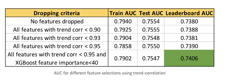
We can see that higher the trend-correlation threshold to drop features, higher is the leaderboard (LB) AUC.
Feature Engineering
The insights that you get by looking at these plots help with creating better features. Just having a better understanding of data can lead to better feature engineering. But, in addition to this, it can also help you in improving the existing features. Let’s look at another feature EXT_SOURCE_1: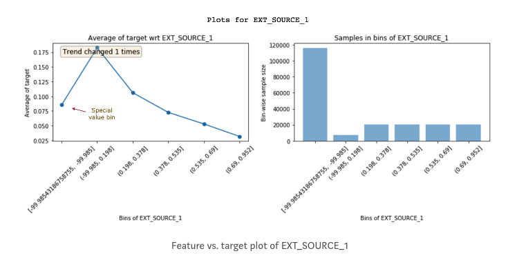
Feature importance
i choose xgboost this part.
Feature debugging
check the trend is or not as you wish.